Excel is supposed to leave the hidden rows alone when you filter a list, select the rows that are left and delete them. Lately, though, Excel has been deleting the hidden rows in between as well for some people, so data they meant to keep is gone, and they only notice when they clear the filter. This guide will explain why it happens and how to delete only the rows you can actually see.
Also see: Excel Copy and Paste Not Working After an Office Update
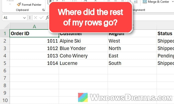
Note: If it just happened, press Ctrl + Z right away. Undo brings every deleted row back, including the hidden ones, as long as you haven’t closed the file.
Why does Excel delete the hidden rows?
Excel treats two kinds of hidden rows very differently. Rows hidden by a filter are normally skipped when you delete, fill or clear a selection, so only the rows you can see are touched. Rows hidden by hand (right-click > “Hide“, by you or someone else who edits the file) are part of the selection like any other row, so deleting rows 2 to 11 deletes all ten of them, whether you can see them or not.
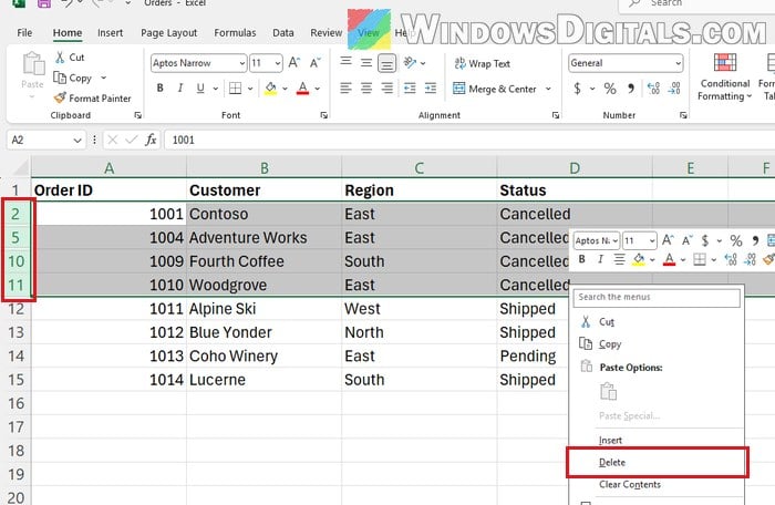
In the example above, only 4 rows are showing between rows 2 and 11, but clicking “Delete” removed all 10 of them, leaving just the rows that came after.
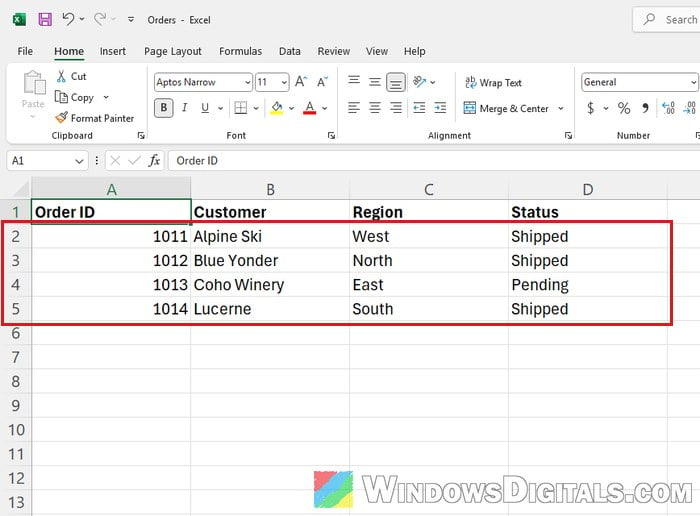
So when the hidden rows get deleted, Excel didn’t treat them as filtered at that moment. Two things can cause that:
- Some rows were hidden by hand before or after the filter, so they aren’t part of the filter at all.
- A recent Microsoft 365 update. Some users started running into this in early November 2026, on sheets where deleting filtered rows had always worked. A recent build may have changed how Excel handles a selection of filtered rows, but Microsoft hasn’t confirmed anything.
Whatever the cause, the fix below should take care of it, since it tells Excel to skip anything hidden.
Related guide: How to Convert CSV or TXT to Excel in Windows 11
Select only the visible cells before you delete
Excel has a built-in way to drop every hidden cell from a selection, whatever hid it. Once you use it, the selection splits into separate blocks around the hidden rows, and deleting it only removes what you can see. Many longtime Excel users do this every time anyway, and it’s the quickest fix.
Here’s how to do it:
- Select the rows you want to delete, the same way you normally would (click the first row number and drag down, or Shift + click the last one).
- Press Alt +
;(semicolon). The selection now shows thin gaps where the hidden rows are.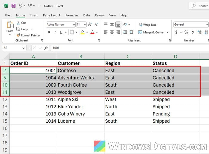
- Right-click one of the selected row numbers and select “Delete” (or “Delete Row” on a filtered list).
- Clear the filter or unhide the rows and check that the hidden rows are still there.
If you prefer the menus, the same selection is in the ribbon:
- Select the rows you want to delete.
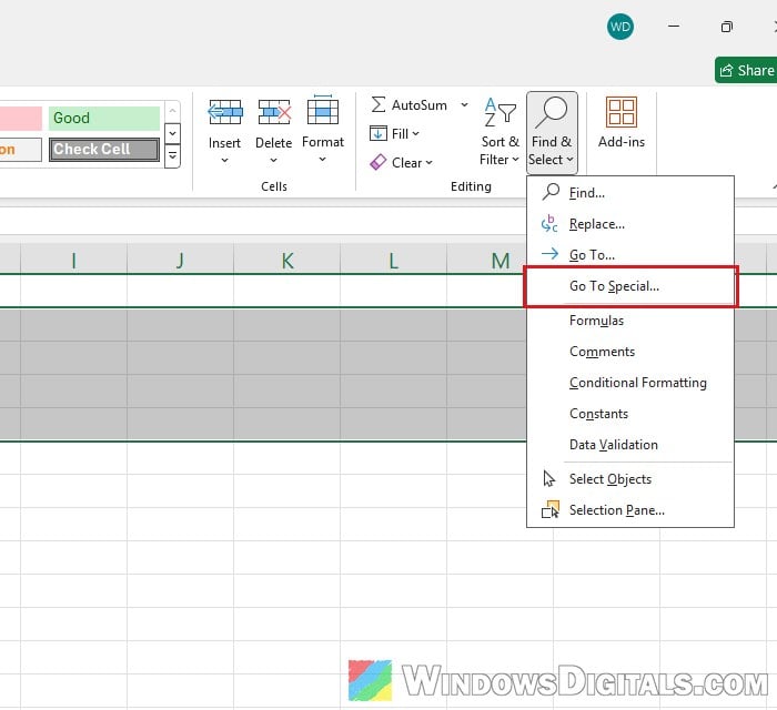
- On the Home tab, click “Find & Select” and choose “Go To Special…“.
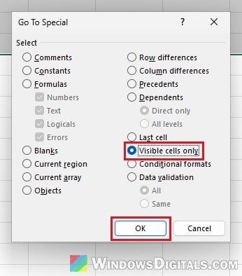
- Select “Visible cells only” and click “OK“.
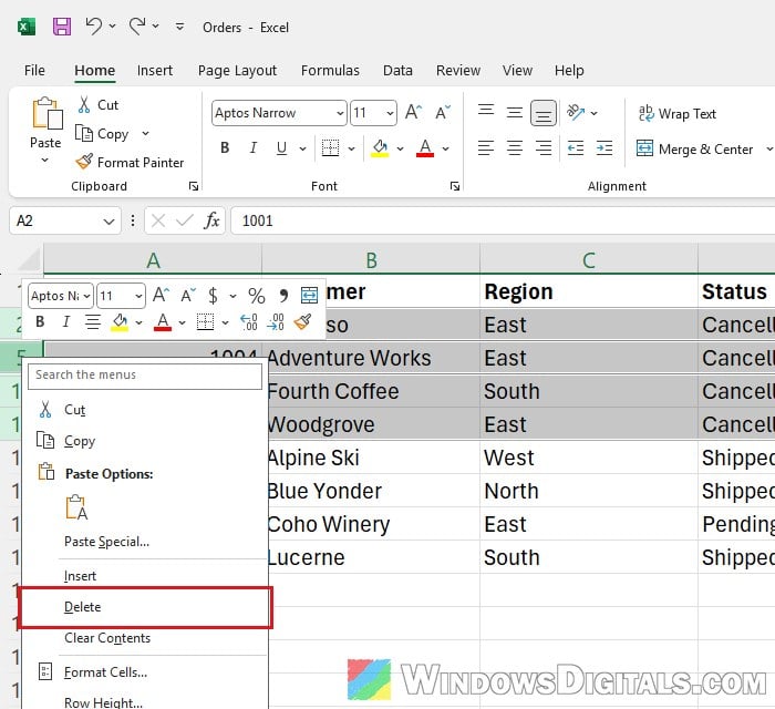
- Right-click a selected row number and select “Delete” (or “Delete Row” on a filtered list).
The same selection works before you copy, too, so only the visible rows end up on the clipboard.
Suggested read: Excel Blocks Macros as Untrusted, How to Enable Them?
Check if the rows are filtered or hidden by hand
If you’d rather not add a step every time, make sure the rows you’re hiding are hidden by the filter alone. It’s easy to tell the two apart. When a filter hides rows, Excel turns the row numbers blue, shows a filter icon on the column you filtered, and the status bar at the bottom says something like “4 of 14 records found“. Rows hidden by hand leave the row numbers black and show no count.
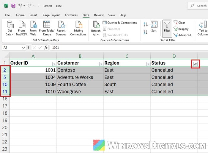
The right-click menu is another giveaway. On rows Excel sees as a filtered list, it offers “Insert Row” and “Delete Row“, and normally, Delete Row only removes the visible rows. If the menu just says “Insert” and “Delete“, Excel is treating the selection as plain rows, and unless you selected visible cells only first, the hidden ones will go too. If your rows are already filtered and the menu says “Delete Row“, but the hidden ones still get deleted, it’s likely the update, so stick with selecting visible cells only.
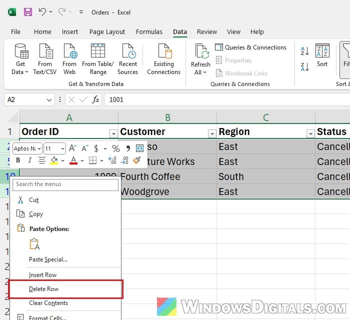
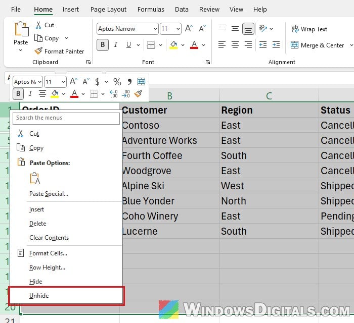
To start clean, unhide everything and let the filter do all the hiding. Here’s what you should do:
- Select all the rows of your list (click the first row number, then Shift + click the last one).
- Right-click a selected row number and select “Unhide“.
- Click any one cell inside the list. Microsoft once documented an Excel bug where turning the filter on with only the header row selected made deletes take the hidden rows too.
- Go to the Data tab and click “Filter” to turn it off, then click “Filter” again to turn it back on.
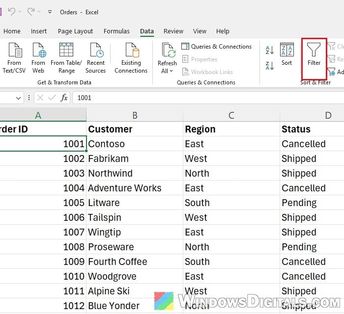
- Set your filter again, select the rows and right-click a row number. You should now see “Delete Row“.
If you add rows later, click “Reapply” next to the Filter button on the Data tab before deleting, so the filter covers the new rows too.
Might be useful: Show or Hide Data Based on a Drop-Down Selection in Excel
Sort the rows together, then delete them in one go
On a big sheet, deleting hundreds of separate blocks of rows can take a while. Sorting avoids the whole issue: if the rows you want gone sit next to each other, there’s nothing hidden between them to delete by mistake, and one solid block deletes much faster.
Follow the steps below:
- If your list has no column that keeps the original order (an ID, a date, a number), add one first and number the rows 1, 2, 3 and so on to the bottom.
- Clear the filter and unhide any rows hidden by hand (steps 1 and 2 in the section above), so nothing hidden is left in the list.
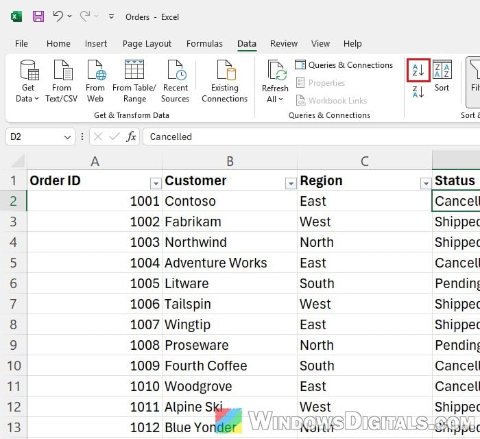
- Click a cell in the column you’d normally filter on, go to the Data tab and click the “Sort A to Z” button (the A-to-Z arrow icon next to “Sort“), or Z to A.
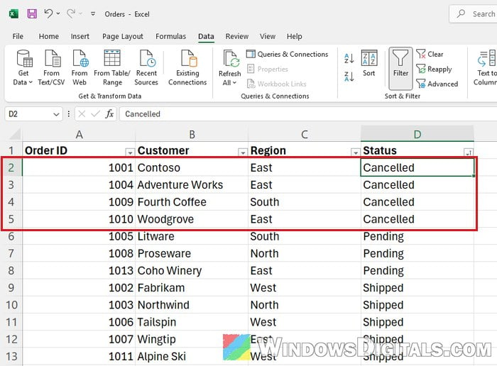
- The rows you want to delete are now together. Select their row numbers and delete them.
- Click a cell in your ID or helper column and sort A to Z again to put the remaining rows back in their original order.
Related concern: Word and Excel Files Turn Into Numbered .tmp Files
Until it’s clear whether a recent update changed anything, clear the filter after any big delete and check the row count before you save.