Show or Hide Data Based on a Drop-Down Selection in Excel

A drop-down list in Excel only controls what can go into its own cell, so picking an item from it won’t make any rows, notes or instructions appear or disappear by itself. To show only the data that matches the choice, you have to connect the drop-down to a formula or a short macro. This guide will help you set that up in a few different ways, from a single formula to actually hiding the rows.

Also see: Excel Copy and Paste Not Working After an Office Update

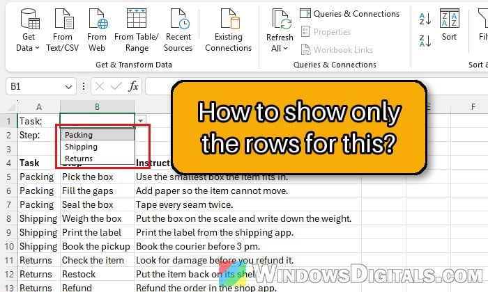
Which method should you use?

It depends on what should happen when someone picks an item:

• Show a copy of only the matching rows: the FILTER function (Excel for Microsoft 365, Excel 2024 or Excel 2021).
• Show a note only for one choice: an IF formula.
• Hide the rows that don’t match: a short macro, which works in older versions too.
• Make a second drop-down offer only the matching choices: FILTER plus a second drop-down.

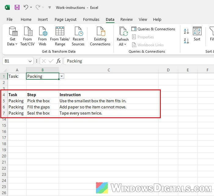
In the examples below, the list (Task, Step and Instruction) has headers in row 4 and data in rows 5 to 13, and the drop-down is in B1. Use your own sheet’s cells instead.

First, create the drop-down list

Every method below reacts to the value in a drop-down cell, so start by creating one with Data Validation:

1. Click the cell where you want the drop-down (B1 in our example).
2. Go to the Data tab and click Data Validation.
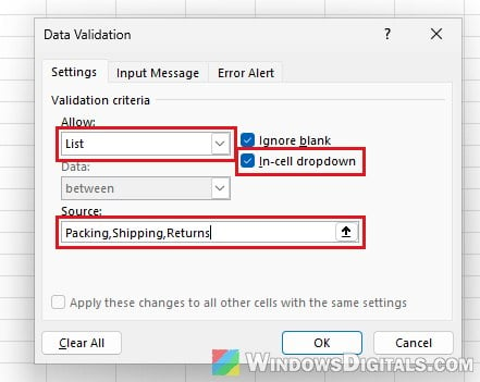
3. On the Settings tab, open the Allow box and select List.
4. Click in the Source box and type the choices separated by commas, such as “Packing,Shipping,Returns“. You can also select a range of cells that holds the list instead (leave out its header).
5. Make sure In-cell dropdown is checked, then click OK.

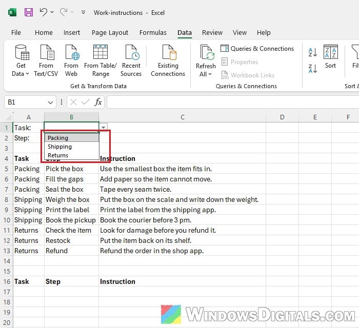
Click the cell again and a small arrow shows the choices.

If the Data Validation button is greyed out, the sheet is probably protected or shared. Unprotect it or stop sharing it, then try again.

Show only the matching rows with the FILTER function

FILTER returns only the rows that meet a condition. When the condition is “the Task column equals the drop-down cell”, the result redraws itself every time someone picks another item. Your list stays as it is, and a live copy of the matching rows shows where the formula is. It’s also what most people asking about this on Reddit ended up using.

1. Copy the header row of your list to where you want the results to show (A16:C16 in our example).
2. Click the cell right below the first header (A17).
3. Type the following formula and press Enter:

   =FILTER(A5:C13,A5:A13=B1,"Nothing to show")

   The first part is the data, the second the condition, and the text at the end shows when nothing matches.
   

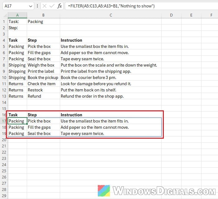
4. Pick another item from the drop-down. The rows under the headers change to match it right away.

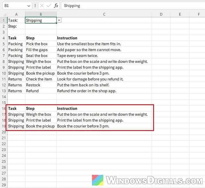
The results “spill” into the cells below and to the right, as many rows as there are matches. Data on another sheet works too, as long as both ranges point to it, such as =FILTER(Data!A5:C13,Data!A5:A13=B1,"Nothing to show").

To filter by two drop-downs at once, multiply the conditions with * (both must match), or add them with + (either one can match), such as =FILTER(A5:C13,(A5:A13=B1)*(B5:B13=B2),"").

What if you see a “#CALC!” or “#SPILL!” error?

#CALC! shows up when nothing matches and the formula has no text for that case (the third part of the formula). #SPILL! means something is in the way of the results, such as a value in one of the cells below or next to the formula. Clear those cells and the results show.

Related problem: VLOOKUP Returns a #SPILL! Error in Excel

Show a note only for one choice with IF

For a line of text that only appears for one item, such as an extra instruction when someone picks “Returns”, an IF formula is enough. It shows the text when the drop-down matches and leaves the cell empty when it doesn’t.

1. Click the cell where the note should show up (C1 in our example).
2. Type a formula like this and press Enter:

   =IF(B1="Returns","Check the item for damage before you refund it.","")

   

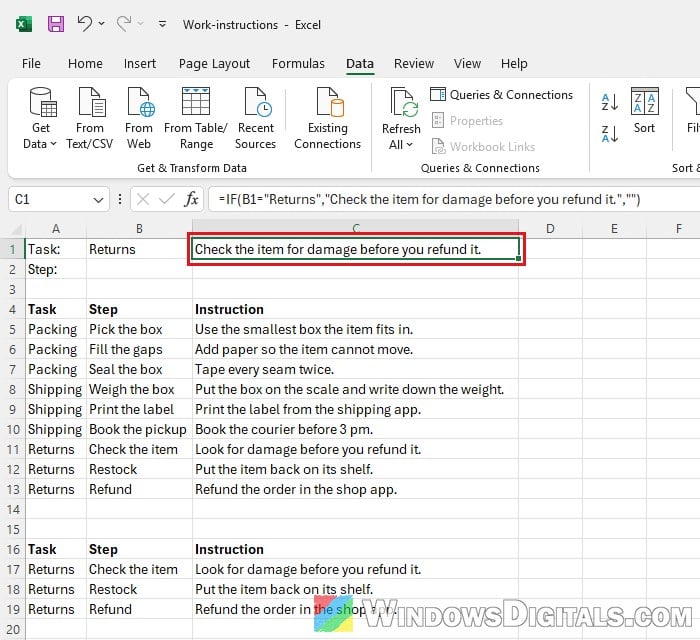
Pick “Returns” and the note shows. Pick anything else and the cell goes blank. If each choice needs its own note, keep the choices and notes in a small table and look them up with XLOOKUP instead of stacking IFs.

Hide the rows that don’t match with a macro

Formulas can show or blank out values, but they can’t hide a row. To hide the rows that don’t belong to the picked item, you need a few lines of VBA that run every time the drop-down changes. This also works in Excel 2019 and older, but only in the desktop app, not Excel for the web.

1. Right-click the sheet’s tab at the bottom of the window and select View Code.
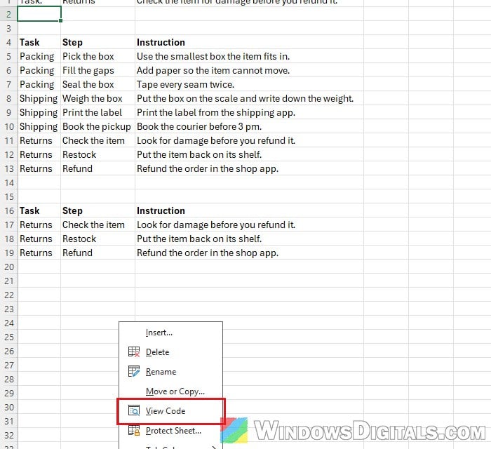
2. In the code window that opens, paste the following:

   Private Sub Worksheet_Change(ByVal Target As Range)
       If Intersect(Target, Range("B1")) Is Nothing Then Exit Sub
       Dim r As Long, v As String
       v = Range("B1").Value
       For r = 5 To 13
           Rows(r).Hidden = (v <> "" And Cells(r, 1).Value <> v)
       Next r
   End Sub

   B1 is the drop-down cell (it appears twice), 5 To 13 are the rows of your list, and Cells(r, 1) is the column to compare (1 is column A). Change them to match your sheet.
   

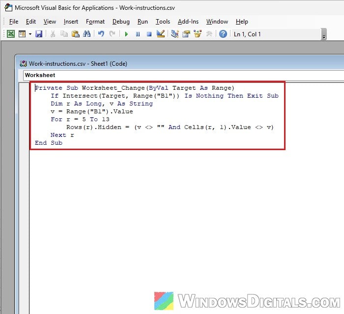
3. Close the code window and go back to the sheet.
4. Pick an item from the drop-down. Only its rows stay visible, and the row numbers on the left skip the hidden ones. Clear the drop-down cell (select it and press Delete) to show every row again.
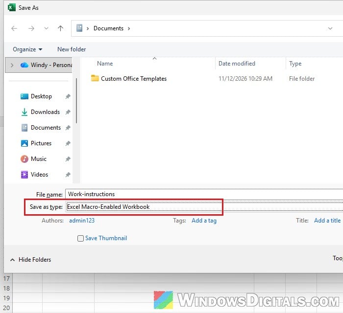
5. Press F12, set Save as type to Excel Macro-Enabled Workbook, and save. A normal .xlsx workbook can’t keep the code.

If you send the file to someone, Excel may block the macro because the file came from the internet or an email.

Might be useful: Excel Blocks Macros as Untrusted, How to Enable Them?

Make a second drop-down show only the matching choices

Sometimes the goal is a second drop-down that only offers what fits the first choice, such as only the steps of the task picked in B1. A FILTER formula builds that short list, and the second drop-down reads from it.

1. In a spare column (E5 in our example), type this formula to list only the steps of the picked task:

   =FILTER(B5:B13,A5:A13=B1,"")

2. Click the cell for the second drop-down (B2), then go to Data > Data Validation.
3. Set Allow to List, and in Source type the formula’s cell followed by a #, such as “=$E$5#“. The # means “the whole list this formula returns”, so the drop-down grows or shrinks with it.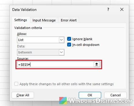
4. Click OK and open the second drop-down. It now only shows the steps that belong to the task in B1.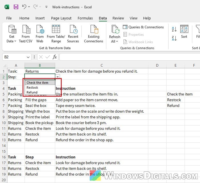

Note: The second cell keeps whatever was picked before, even after the first choice changes. Clear it and pick again when you switch the first drop-down.

Using Excel 2019 or older?

FILTER isn’t in Excel 2019 or older, so on those versions the macro above is the only way to make a drop-down change which rows show. Without a macro, Excel’s built-in filter does a similar job by hand:

1. Click any cell in your list and go to Data > Filter.
2. Click the arrow on the Task header.
3. Untick (Select All), tick only the item you want to see, and click OK.

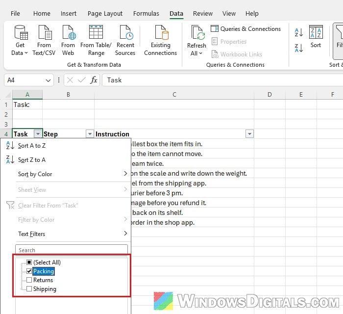
It isn’t tied to a drop-down cell, but it hides the other rows, and clearing the filter brings them back.